Component models¶

The component models of the open-plan-tool result from the used python-library oemof-solph for energy modeling.

It requires component models to be simplified and linearized. This is the reason why the open-plan-tool can provide a pre-feasibility study of a specific system setup, but not the final sizing and system design. The types of assets are presented below.

Energy consumption¶

Demands within the open-plan-tool are added as energy consumption assets. Most importantly, they are defined by a timeseries, representing the demand profile, and their energy vector. A number of demand profiles can be defined for one energy system, both of the same and different energy vectors. The main optimization goal for the open-plan-tool is to supply the defined demand without fail for all of the timesteps in the simulation with the least cost of supply (comp. Economic Dispatch).

Energy production¶

Non-dispatchable sources of generation¶

Examples:

PV plants

Wind plants

Run-of-the-river hydro power plants

Solar thermal collectors

Variable renewable energy (VRE) sources, like wind and PV, are non-dispatchable due to their fluctuations in supply.

The fluctuating nature of non-dispatchable sources is represented by generation time series that show the respective production for each time step of the simulated period. In energy system modelling it is common to use hourly time series.

If you cannot provide time series for your VRE assets you can consider to calculate them by using models for generating feed-in time series from weather data. The following is a list of examples, which is not exhaustive:

PV: pvlib , Renewables Ninja (download capacity factors), altlite

Wind: windpowerlib, Renewables Ninja (download capacity factors), altlite

Hydro power (run-of-the-river): hydropowerlib

Solar thermal: flat plate collectors of oemof.thermal

Dispatchable sources of generation¶

Examples:

Fuel sources

Deep-ground geothermal plant (ground assumed to allow unlimited extraction of heat, not depending on season)

Fuel sources are added as dispatchable sources, which can have development, investment, operational and dispatch costs.

Fuel sources are for example needed as source for a diesel generator (diesel), biogas plant (gas) or a condensing power plant (gas, coal, …), see Energy conversion.

Energy conversion¶

Examples:

Electric transformers (rectifiers, inverters, transformer stations, charge controllers)

HVAC and Heat pumps (as heater and/or chiller)

Combined heat and power (CHP) and other condensing power plants

Diesel generators

Electrolyzers

Biogas power plants

Conversion assets are added as transformers.

The parameters dispatch_price, efficiency and installedCap of transformers are assigned to their output flows. This means that these parameters need to be provided for the output of the asset and that the costs of the input, (e.g. cost of fuel) are not included in its dispatch_price but in the dispatch_price of the fuel source, see Dispatchable sources of generation.

Conversion assets can be defined with multiple inputs or multiple outputs, but one asset currently cannot have both, multiple inputs and multiple outputs. Note that multiple inputs/output is possible but this feature is not currently tested.

Electric transformers¶

Electric rectifiers and inverters that are transforming electricity in one direction only, are simply added as transformers. Bidirectional converters and transformer stations are defined by two transformers that are optimized independently from each other, if optimized. The same accounts for charge controllers for a Battery energy storage system (BESS) that are defined by two transformers, one for charging and one for discharging. The parameters dispatch_price, efficiency and installedCap need to be given for the electrical output power of the electric transformers.

Note

When using two conversion objects to emulate a bidirectional conversion asset, their capacity should be interdependent. This is currently not the case, see Infeasible bi-directional flow in one timestep.

Heating, Ventilation, and Air Conditioning (HVAC)¶

Like other conversion assets, devices for heating, ventilation and air conditioning (HVAC) are added as transformers. As the parameters dispatch_price, efficiency and installedCap are assigned to the output flows they need to be given for the nominal heat output of the HVAC.

Different types of HVAC can be modelled. Except for an air source device with ambient temperature as heat reservoir, the device could be modelled with two inputs (electricity and heat) in case the user is interested in the heat reservoir. This has not been tested yet. Also note that currently efficiencies are assigned to the output flows the see issue #799. Theoretically, a HVAC device can be modelled with multiple outputs (heat, cooling, …); this has not been tested yet.

The efficiency of HVAC systems is defined by the coefficient of performance (COP), which is strongly dependent on the temperature. In order to take account of this, the efficiency can be defined as time series. If you do not provide your own COP time series you can calculate them with oemof.thermal, see documentation on compression heat pumps and chillers and documentation on absorption chillers.

Electrolyzers¶

Electrolyzers are added as transformers with a constant or time dependent but in any case pre-defined efficiency. The parameters dispatch_price, efficiency and installedCap need to be given for the output of the electrolyzers (hydrogen).

Currently, electrolyzers are modelled with only one input flow (electricity), not taking into account the costs of water; see issue #799. The minimal operation level and consumption in standby mode are not taken into account, yet, see issue #50.

Condensing power plants and Combined heat and power (CHP)¶

Condensing power plants are added as transformers with one input (fuel) and one output (electricity), while CHP plants are defined with two outputs (electricity and heat). The parameters dispatch_price, efficiency and installedCap need to be given for the electrical output power (and nominal heat output) of the power plant, while fuel costs need to be included in the dispatch_price of the fuel source.

The ratio between the heat and electricity output of a CHP is currently simulated as fix values. This might be changed in the future by using the ExtractionTurbineCHP or the GenericCHP component of oemof, see issue #803

Note that multiple inputs/output have not been tested yet.

Other fuel powered plants¶

Fuel powered conversion assets, such as diesel generators and biogas power plants, are added as transformers. The parameters dispatch_price, efficiency and installedCap need to be given for the electrical output power of the diesel generator or biogas power plant. As described above, the costs for diesel and gas need to be included in the dispatch_price of the fuel source.

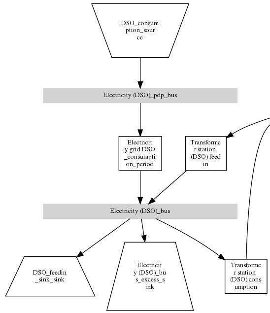
Energy providers¶

The energy providers are the most complex assets in the open-plan-tool model. They are composed of a number of sub-assets

Energy consumption source, providing the energy required from the system with a certain price

Energy peak demand pricing “transformers”, which represent the costs induced due to peak demand

Bus connecting energy consumption source and energy peak demand pricing transformers

Energy feed-in sink, able to take in generation that is provided to the energy provider for revenue

Optionally: Transformer Station connecting the energy provider bus to the energy bus of the LES

With all these components, the energy provider can be visualized as follows:

../_images/Model_Assumptions_energyProvider_assets.png

Variable energy consumption prices (time-series)¶

Energy consumption prices can be added as values that vary over time.

Peak demand pricing¶

A peak demand pricing scheme is based on an electricity tariff, that requires the consumer not only to pay for the aggregated energy consumption in a time period (eg. kWh electricity), but also for the maximum peak demand (load, eg. kW power) towards the grid of the energy provider within a specific pricing period.

In the open-plan-tool, this information is gathered in the provider assets with:

multi_vector_simulator.utils.constants_json_strings.PEAK_DEMAND_PRICING_PERIOD as the period used in peak demand pricing. Possible values are 1 (yearly), 2 (half-yearly), 3 (each trimester), 4 (quaterly), 6 (every 2 months) and 12 (each month). If you have a simulation_duration < 365 days, the periods will still be set up assuming a year! This means, that if you are simulating 14 days, you will never be able to have more than one peak demand pricing period in place.

multi_vector_simulator.utils.constants_json_strings.PEAK_DEMAND_PRICING as the costs per peak load unit, eg. kW

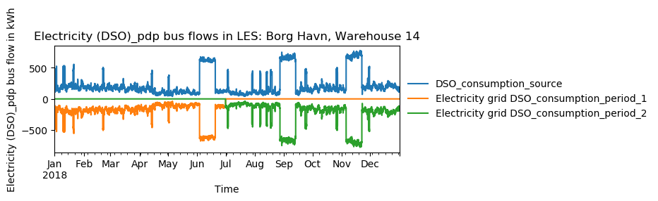
To represent the peak demand pricing, the open-plan-tool adds a “transformer” that is optimized with specific operation and maintenance costs per year equal to the PEAK_DEMAND_PRICING for each of the pricing periods. For two peak demand pricing periods, the resulting dispatch could look as following:

../_images/Model_Assumptions_Peak_Demand_Pricing_Dispatch_Graph.png

Energy storage¶

Energy storages such as battery storages, thermal storages or H2 storages are modelled with the GenericStorage component of oemof.solph. They are designed for one input and one output.

The state of charge of a storage at the first and last time step of an optimization are equal. Charge and discharge of the whole capacity of the energy storage are possible within one time step in case the capacity of the storage is not optimized. In case of capacity optimization charge and discharge is limited by the c-rate.

Battery energy storage system (BESS)¶

BESS are modelled as GenericStorage like described above. The BESS can either be connected directly to the electricity bus of the LES or via a charge controller that manages the BESS. When choosing the second option, the capacity of the charge controller can be optimized individually, which takes its specific costs and lifetime into consideration. A charge controller is defined by two transformers, see section Energy conversion above.

Note that capacity reduction over the lifetime of a BESS that may occur due to different effects during aging cannot be taken into consideration in the open-plan-tool. A possible workaround for this could be to manipulate the lifetime.

Hydrogen storage (H2)¶

Hydrogen storages are modelled as all storage types in the open-plan-tool as GenericStorage like described above.

The most common hydrogen storages store H2 as liquid under temperatures lower than -253 °C or under high pressures. The energy needed to provide these requirements cannot be modelled via the storage component as another energy sector such as cooling or electricity is needed. It could therefore, be modelled as an additional demand of the energy system, see issue #811

Thermal energy storage¶

Thermal energy storages of the type sensible heat storage (SHS) are modelled as GenericStorage like described above. The implementation of a specific type of SHS, the stratified thermal energy storage, is described in section Stratified thermal energy storage. The modelling of latent-heat (or Phase-change) and chemical storages have not been tested with the open-plan-tool, but might be achieved by precalculations.

Stratified thermal energy storage¶

Stratified thermal energy storage is defined by the two optional parameters fixed_thermal_losses_relative and fixed_thermal_losses_absolute. These two parameters are used to take into account temperature dependent losses of a thermal storage. To model a thermal energy storage without stratification, the two parameters are not set. The default values of fixed_thermal_losses_relative and fixed_thermal_losses_absolute are zero. Except for these two additional parameters the stratified thermal storage is implemented in the same way as other storage components.

Precalculations of the installedCap, efficiency, fixed_thermal_losses_relative and fixed_thermal_losses_absolute can be done orientating on the stratified thermal storage component of oemof.thermal. The parameters U-value, volume and surface of the storage, which are required to calculate installedCap, can be precalculated as well.

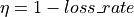
The efficiency $\eta$ of the storage is calculated as follows:

$\eta = 1 - loss{\_}rate$

This example shows how to do precalculations using stratified thermal storage specific input data:

from oemof.thermal.stratified_thermal_storage import (
calculate_storage_u_value,
calculate_storage_dimensions,
calculate_capacities,
calculate_losses,
)

# Precalculation
u_value = calculate_storage_u_value(
    input_data['s_iso'],
    input_data['lamb_iso'],
    input_data['alpha_inside'],
    input_data['alpha_outside'])

volume, surface = calculate_storage_dimensions(
    input_data['height'],
    input_data['diameter']
)

nominal_storage_capacity = calculate_capacities(
    volume,
    input_data['temp_h'],
    input_data['temp_c'])

loss_rate, fixed_losses_relative, fixed_losses_absolute = calculate_losses(
    u_value,
    input_data['diameter'],
    input_data['temp_h'],
    input_data['temp_c'],
    input_data['temp_env'])

Please see the oemof.thermal examples and the documentation for further information.

For an investment optimization the height of the storage should be left open in the precalculations and installedCap should be set to 0 or NaN.

An implementation of the stratified thermal storage component has been done in pvcompare. You can find the precalculations of the stratified thermal energy storage made in pvcompare here.

Energy excess¶

Note

Energy excess components are implemented automatically by the open-plan-tool! You do not need to define them yourself.

An energy excess sink is placed on each of the LES energy busses, and therefore energy excess is allowed to take place on each bus of the LES. This means that there are assumed to be sufficient vents (heat) or resistors (electricity) to dump excess (waste) generation. Excess generation can only take place when a non-dispatchable source is present or if an asset is allowed to supply energy without any fuel or dispatch costs.

In case of excessive excess energy, a warning is issued that it seems to be cheaper to have high excess generation than investing into more capacities. High excess energy can for example result into an optimized inverter capacity that is smaller than the peak generation of installed PV. The model becomes unrealistic when the excess is very high.