The mathematics behind open-plan-tool simply explained
Aim of the open-plan-tool
The aim of the open-plan-tool is to provide an open source application that has the capability to model small to medium-sized energy systems with emphasis on renewable energy technologies and optimize them cost-efficiently. The easy to use graphical user interface and also the in-depth insight into the optimization program and its visible open source code encourages end-users and also researchers to use it. .. [Write some more about the aim of open-plan-tool…..]
One important aspect of future scenarios is the determination of optimal dimensioning and combinations of various technologies. To compute an optimal individual energy system open-plan-tool uses linear optimization. When we think about how we want to set up our energy system, we have several goals. For example, we want to minimize the cost of the energy system or the amount of CO2 that we emit. Furthermore, we want to make sure that demand can be met at any point in time, as well as a variety of other goals. To help us find a way to satisfy all these goals, we can use linear optimization. What was briefly outlined in the last section is basically a non-mathematical way of describing the main and secondary conditions that we need to use linear optimization. In the following example, this will be further illustrated.
[Das folgende ist ein einfaches Beispiel, was die Methodik der linearen Optimierung anhand eines zweidimensionalen Lösungsraums erklären soll.] The following example describes the principle of linear optimization in a two-dimensional space.
An energy system with various technologies
When it comes to electricity generation, we can imagine a simple energy system using solar energy and fossil fuels. To use solar energy we need PV modules, and to use the fossil fuel, we need a fossil fuel power station. For both technologies we are trying to find out how much capacity we should build to get the cost minimum solution. We also have a battery and we have the consumer for which we know the exact demand.
[Picture Energysystem]
Using this data, we can now think about our optimal solution. In this case our objective is to minimize costs. The objective function is described as a linear function that we want to minimize. [spez. Kosten + repective installed capacities]
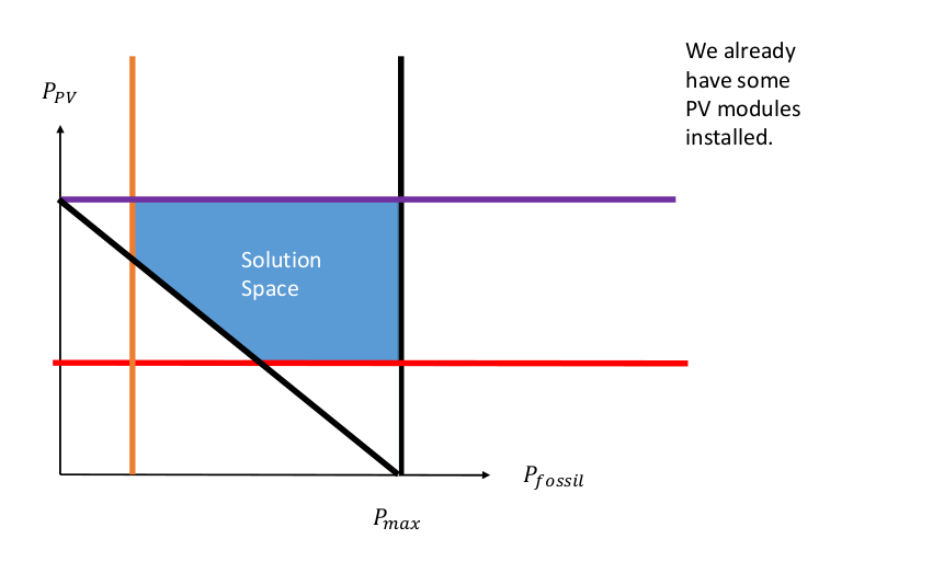
We can now represent this graphically as a solution space, which shows us all the possible input combinations. On the x-axis we have the fossil fuel generator capacity, and on the y-axis we have the capacity of a PV plant. Any point within the solution space is a possible solution, and using linear optimization, we will find the optimum.
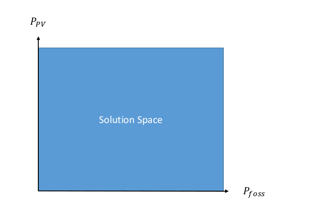
If we just want to minimize the costs, we would have to say that the optimum is (0,0), as this costs us the least. Therefore, we need to add more information, or more secondary conditions. An optimization is linear as long as the main and secondary conditions only contain linear functions. In the following section, we will look at a few secondary conditons.
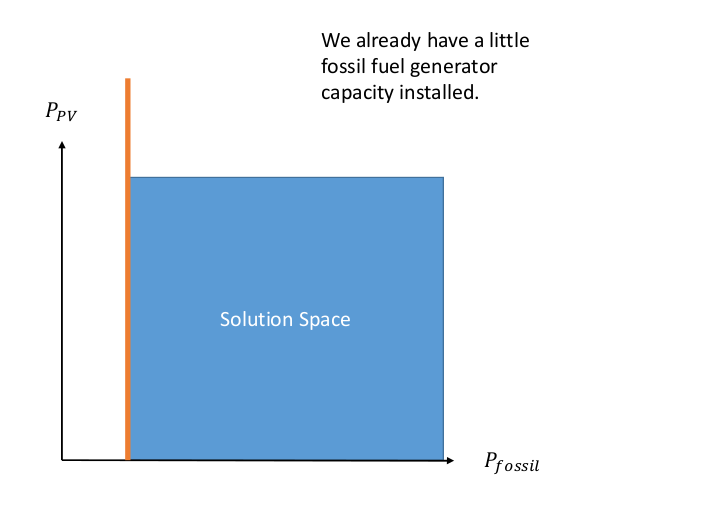
In our example, we assume that a small fossil fuel generator has already been installed, and consequently, the solution space is reduced, as shown in the picture.
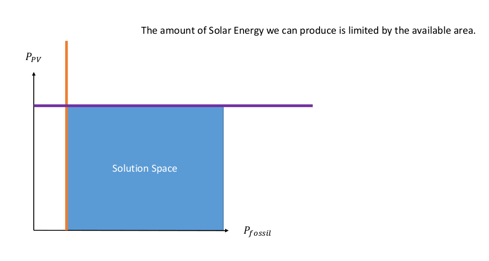
Another secondary condition is that the amount of solar capacity that we can build is restricted by the area that we can actually build solar cells on, which is represented by the purple line.
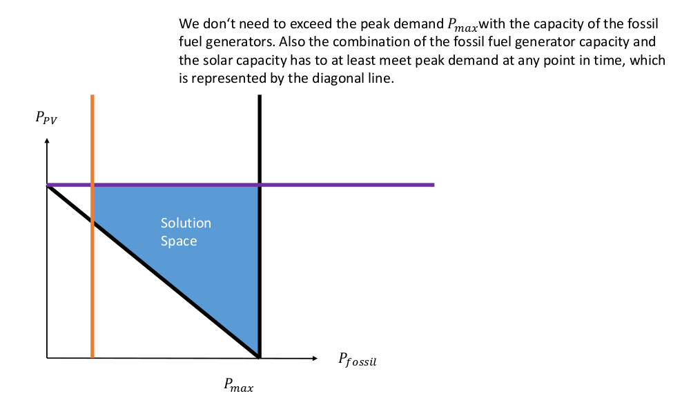
We also know that we do not want to install more capacity than necessary, meaning that the generation capacity of the fossil fuel generator should not exceed the peak demand, which is shown by the black straight line.
We also have to be able to meet the peak demand. We need to make sure that we have enough capacity installed to meet this demand, which is depicted by the diagonal line, which shows us all the combinations of solar and fossil fuel capacity that let us meet peak demand. However, all the solutions above the diagonal line are also theoretically possible.
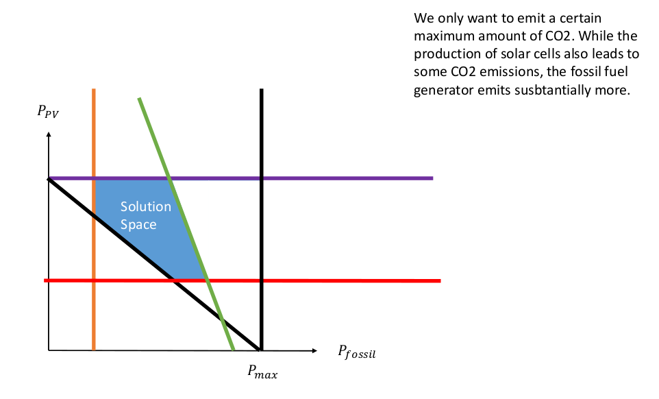
We also have some PV plants installed and consequently our solution space is reduced again.
Finally, we also want to make sure that our energy system is sustainable, and therefore, we define a maximum amount of CO2 that we want to emit, which is represented by the green line. After having reduced the solution space again, we now turn to solving the optimization problem.
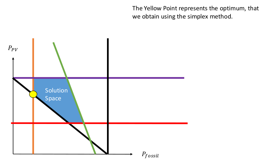
After we have defined our solution space, the next step is to find the optimum. Several ways of solving these problems have been developed, one of which is the simplex method. This can be done on paper, but as the number of equations rises, this becomes more and more difficult.
In open-plan-tool this is done by a solver, which can solve the optimization, given that the equations are in a certain form. The solver then proceeds in two steps. In the first step, it checks if there is a solution to the problem, and as soon as a solution is found, the solver proceeds to the second step. In the second step, the solver then tries to find a better solution and continues this process iteratively until it has found the best solution. To do this, the solver moves along the edges of the solutions space, as the optimum will always lie on the edge of the solution space in a linear optimization model as long as there is an optimum. In our simple example, this means that the solution has to lie somewhere on the edge of our solutions space. In this case the solution is the yellow point.
It is also possible that several solutions exist. Graphically, this would mean that an entire edge of the constraint to the solution space would be an optimum, meaning that we have several solutions that give us the same optimal result. In this case we can pick any point of the input combinations that lead us to the optimal solution. If we increase the complexity, by either adding more secondary conditions, or by expanding the main condition, the solution space becomes more complex, and can go from 3 Dimensional to 50 Dimensional or even more. When the solution space becomes more complex, it becomes basically impossible to graphically demonstrate how the solution space is solved, but the principle is exactly the same in a two dimensional problem or a 50 dimensional problem, it just takes longer for the solver to do its work.