Assumptions¶

The open-plan-tool uses the programming framework oemof-solph at its core and builds an energy system model based upon its nomenclature. As such, the energy system model can be described with a linear equation system. The most important aspects of a linear equation system are described below in a generalized way, and additionally explained through the use of an example. This will enable the clear comparision to other energy system models.

Economic Dispatch¶

Linear programming is a mathematical modelling and optimization technique for a system of a linear objective function subject to linear constraints. The goal of a linear programming problem is to find the optimal value for the objective function, be it a maximum or a minimum. open-plan-tool is based on oemof-solph, which in turn uses Pyomo to create a linear problem. The economic dispatch problem in the open-plan-tool has the objective of minimizing the production cost by allocating the total demand among the generating units at each time step. The equation is the following:

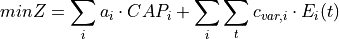
$min Z = \sum_i a_i \cdot CAP_i + \sum_i \sum_t c_{var,i} \cdot E_i(t)$

$CAP_i &\geq 0 E_i(t) &\geq 0 \qquad \forall t i &\text{: asset} a_i &\text{: asset annuity [currency/kWp/year, currency/kW/year, currency/kWh/year]} CAP_i &\text{: asset capacity [kWp, kW, kWh]} c_{var,i} &\text{: variable operational or dispatch cost [currency/kWh, currency/L]} E_i(t) &\text{: asset dispatch [kWh]}$

The annual cost function of each asset includes the capital expenditure (investment cost) and residual value, as well as the operating expenses of each asset. It is expressed as follows:

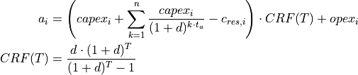
$a_i &= \left( capex_i + \sum_{k=1}^{n} \frac{capex_i}{(1+d)^{k \cdot t_a}} - c_{res,i} \right) \cdot CRF(T) + opex_i CRF(T) &= \frac{d \cdot (1+d)^T}{(1+d)^T - 1}$

$capex_i &\text{: specific investment costs [currency/unit]} n &\text{: number of replacements of an asset within project lifetime } T t_a &\text{: asset lifetime [years]} CRF &\text{: capital recovery factor} c_{res,i} &\text{: residual value of asset i at the end of project lifetime } T \text{ [currency/unit]} opex_i &\text{: annual operational and management costs [currency/unit/year]} d &\text{: discount factor} T &\text{: project lifetime [years]}$

The CRF is a ratio used to calculate the present value of the annuity. The discount factor can be replaced by the weighted average cost of capital (WACC), calculated by the user.

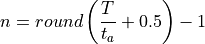
The lifetime of the asset $t_a$ and the lifetime of the project $T$ can be different from each other; as a result, the number of replacements $n$ is estimated using the equation below:

$n = round \left( \frac{T}{t_a} + 0.5 \right) - 1$

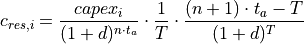
The residual value is also known as the salvage value and it represents an estimate of the monetary value of an asset at the end of the project lifetime $T$ . open-plan-tool considers a linear depreciation over $T$ and accounts for the time value of money through the use of the following equation:

$c_{res,i} = \frac{capex_i}{(1+d)^{n \cdot t_a}} \cdot \frac{1}{T} \cdot \frac{(n+1) \cdot t_a - T}{(1+d)^T}$

Energy Balance Equation¶

One main constraint that the optimization model is subject to is the energy balance equation, which specifically maintains equality between the total incoming and outgoing energy of a bus. This balancing equation is applicable to all bus types, be it electrical, thermal, hydrogen or any other energy carrier.

$\sum E_{in,i}(t) - \sum E_{out,j}(t) = 0 \qquad \forall t$

$E_{in,i} &\text{: energy flowing from asset i to the bus} E_{out,j} &\text{: energy flowing from the bus to asset j}$

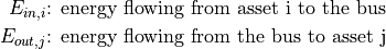
It is very important to note that assets i and j can be the same asset (e.g. a battery with an electrical inflow/outflow). Oemof-solph allows both $E_{in}$ and $E_{out}$ to be larger than zero in the same time step t (see Infeasible bi-directional flow in one timestep).

Example: Sector Coupled Energy System¶

In order to understand the component models, a generic sector coupled energy system example is shown in the figure below. It brings together the electricity and heat sector through a transformer (Transformer 4) which connects the two sector buses.

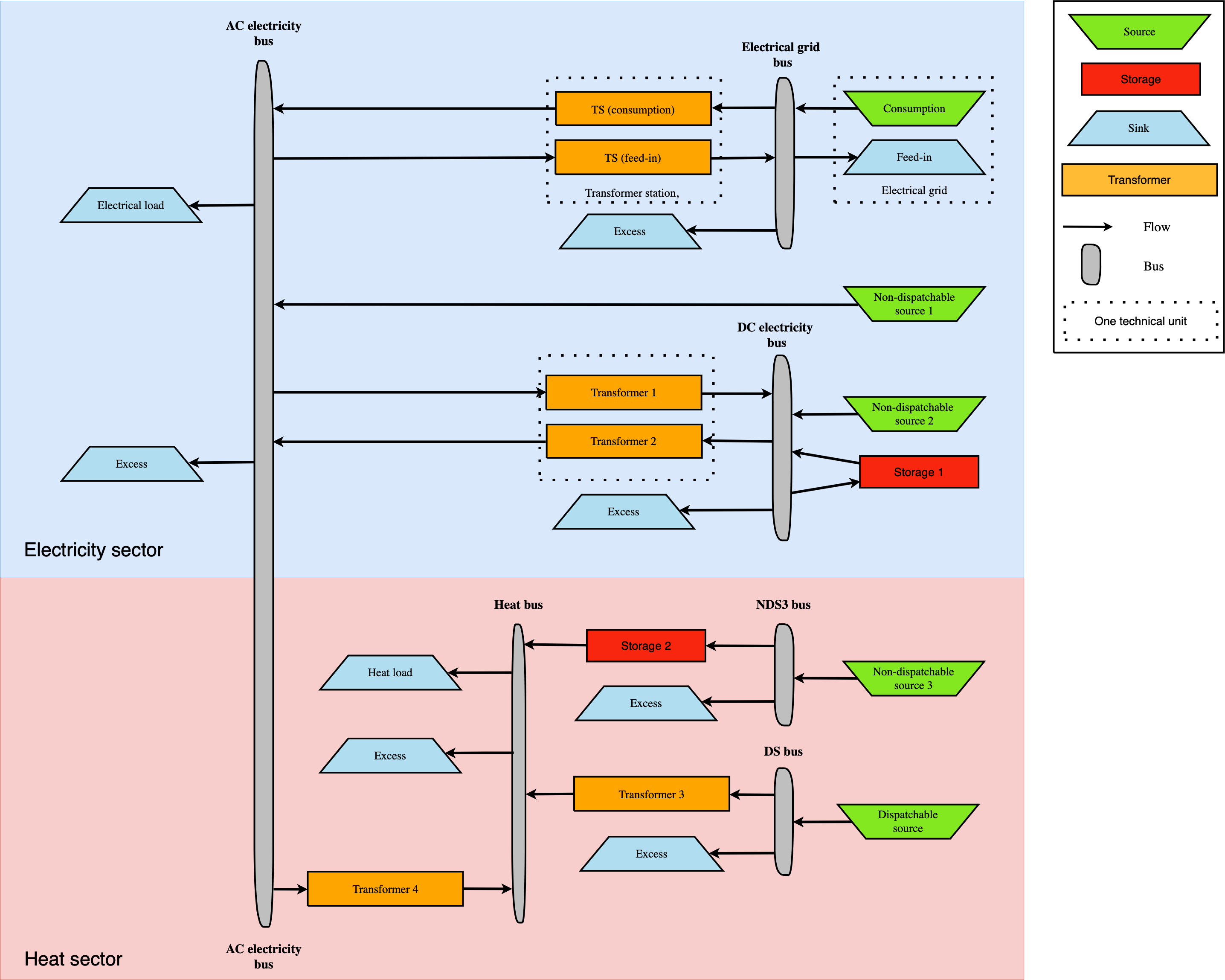
../_images/26-10-2020_sector_coupled_example.png

For the sake of simplicity, the following table gives an example for each asset type with an abbreviation to be used in the energy balance and component equations.

Asset Types and Examples¶

Asset Type

Asset Example

Abbreviation

Unit

Non-dispatchable source 1

Wind turbine

wind

kW

Non-dispatchable source 2

Photovoltaic panels

pv

kWp

Storage 1

Battery energy storage

bat

kWh

Transformer 1

Rectifier

rec

kW

Transformer 2

Solar inverter

inv

kW

Non-dispatchable source 3

Solar thermal collector

stc

kWth

Storage 2

Thermal energy storage

tes

kWth

Dispatchable source

Heat source (e.g., biogas)

heat

L

Transformer 3

Turbine

turb

kWth

Transformer 4

Heat pump

hp

kWth

All grid and dispatchable source asset types are assumed to be available 100% of the time with no consumption limits. For each bus in the system, the open-plan-tool automatically includes a sink component for excess energy related to the bus, which is denoted $E_{ex}$ in the equations. This excess sink accounts for the extra energy in the system that has to be dumped.

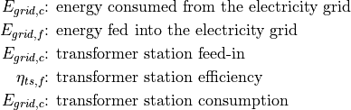
Electricity Grid Equation¶

The electricity grid is modeled through a feed-in and a consumption node. Transformers limit the peak flow into or from the local electricity line, and electricity sold to the grid experiences losses in the transformer $(ts,f)$ .

$E_{grid,c}(t) - E_{grid,f}(t) + E_{ts,f}(t) \cdot \eta_{ts,f} - E_{ts,c}(t) = 0 \qquad \forall t$

$E_{grid,c} &\text{: energy consumed from the electricity grid} E_{grid,f} &\text{: energy fed into the electricity grid} E_{grid,c} &\text{: transformer station feed-in} \eta_{ts,f} &\text{: transformer station efficiency} E_{grid,c} &\text{: transformer station consumption}$

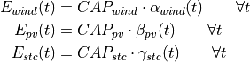
Non-Dispatchable Source Equations¶

Non-dispatchable sources in the sector coupled energy system example are wind, PV and solar thermal power. Their generation is determined by the provided timeseries of instantaneous generation, providing $\alpha$ , $\beta$ , $\gamma$ in relation to wind, PV and solar thermal power respectively.

$E_{wind}(t) &= CAP_{wind} \cdot \alpha_{wind}(t) \qquad \forall t E_{pv}(t) &= CAP_{pv} \cdot \beta_{pv}(t) \qquad \forall t E_{stc}(t) &= CAP_{stc} \cdot \gamma_{stc}(t) \qquad \forall t$

$E_{wind} &\text{: energy generated from the wind turbine} CAP_{wind} &\text{: wind turbine capacity [kW]} \alpha_{wind} &\text{: instantaneous wind turbine performance metric [kWh/kW]} E_{pv} &\text{: energy generated from the PV panels} CAP_{pv} &\text{: PV panel capacity [kWp]} \beta_{pv} &\text{: instantaneous PV specific yield [kWh/kWp]} E_{stc} &\text{: energy generated from the solar thermal collector} CAP_{stc} &\text{: Solar thermal collector capacity [kWth]} \gamma_{stc} &\text{: instantaneous collector's production [kWh/kWth]}$

Storage Model¶

There are two storages in the defined example system: An electrical energy storage (Storage 1, $bat$ ) and a thermal energy storage (Storage 2, $tes$ ). Below, the equations for Storage 1 are provided, but Storage 2 follows analogous equations for charge, discharge and bounds.

$E_{bat}(t) = E_{bat}(t - 1) + E_{bat,in}(t) \cdot \eta_{bat,in} - \frac{E_{bat,out}}{\eta_{bat,out}} - E_{bat}(t - 1) \cdot \epsilon \qquad \forall t$

$CAP_{bat} \cdot SOC_{min} \leq E_{bat}(t) \leq CAP_{bat} \cdot SOC_{max} \qquad \forall t 0 \leq E_{bat}(t) - E_{bat}(t - 1) \leq CAP_{bat} \cdot C_{rate,in} \qquad \forall t 0 \leq E_{bat}(t - 1) - E_{bat}(t) \leq CAP_{bat} \cdot C_{rate,out} \qquad \forall t$

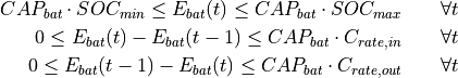
$E_{bat} &\text{: energy stored in the battery at time t} E_{bat,in} &\text{: battery charging energy} \eta_{bat,in} &\text{: battery charging efficiency} E_{bat,out} &\text{: battery discharging energy} \eta_{bat,out} &\text{: battery discharging efficiency} \epsilon &\text{: decay per time step} CAP_{bat} &\text{: battery capacity [kWh]} SOC_{min} &\text{: minimum state of charge} SOC_{max} &\text{: maximum state of charge} C_{rate,in} &\text{: battery charging rate} C_{rate,in} &\text{: battery discharging rate}$

DC Electricity Bus Equation¶

The following equation illustrates an example of a DC bus with a battery, PV and a bi-directional inverter.

$E_{pv}(t) + E_{bat,out}(t) \cdot \eta_{bat,out} + E_{rec}(t) \cdot \eta_{rec} - E_{inv}(t) - E_{bat,in} - E_{ex}(t) = 0 \qquad \forall t$

$E_{rec} &\text{: rectifier energy} \eta_{rec} &\text{: rectifier efficiency} E_{inv} &\text{: inverter energy}$

AC Electricity Bus Equation¶

This equation describes the local electricity grid and all connected assets:

$E_{ts,c}(t) \cdot \eta_{ts,c} + E_{wind}(t) + E_{inv}(t) \cdot \eta_{inv} - E_{ts,c}(t) - E_{rec}(t) - E_{hp}(t) - E_{el}(t) - E_{ex}(t) = 0 \qquad \forall t$

$\eta_{ts,c} &\text{: transformer station efficiency} \eta_{inv} &\text{: inverter efficiency} E_{hp} &\text{: heat pump electrical consumption} E_{el} &\text{: electrical load}$

Heat Bus Equation¶

This equation describes the heat bus and all connected assets:

$E_{tes}(t) \cdot \eta_{tes} + E_{turb}(t) \cdot \eta_{turb} + E_{hp}(t) \cdot COP - E_{th}(t) - E_{ex}(t) = 0$

$\eta_{tes} &\text{: thermal storage efficiency} \eta_{turb} &\text{: turbine efficiency} COP &\text{: heat pump coefficient of performance} E_{th} &\text{: heat load}$

NDS3 Bus Equation¶

The NDS3 Bus is an example of a bus which does not serve both as the input and output of a storage system. Instead, the thermal storage is charged from the NDS3 bus, but discharges into the heat bus.

$E_{stc}(t) - E_{tes}(t) - E_{ex}(t) = 0$

$E_{tes} \text{: thermal energy storage}$

DS Bus Equation¶

The DS Bus shows an example of a fuel source providing an energy carrier (biogas) to a transformer (turbine).

$E_{heat}(t) - E_{turb}(t) - E_{ex}(t) = 0$

$E_{heat} &\text{: thermal energy (biogas) production} E_{turb} &\text{: turbine (biogas turbine) energy}$

Cost calculations¶

The optimization of the open-plan-tool is mainly based on costs. There is, however, the possibility of introducing additional constraints which will impact the optimization results e.g. implementing a maximum installable capacity limit (comp. maximumCap) or adding constraints for certain key performance indicators (see Constraints). In order to optimize the energy systems properly, the economic data provided with the input data has to be pre-processed (also see Economic Dispatch) and then also post-processed when evaluating the results. The following assumptions are therefore important:

Project lifetime: The simulation has a defined project lifetime, for which continuous operation is assumed - which means that the first year of operation is considered to be the same as the last year of operation. Existing and optimized assets have to be replaced (if their lifetime preceeds the system lifetime) to make this possible.
Simulation duration: It is advisable to simulate the whole year to find the most suitable combination of energy assets for your system. Sometimes however you might want to look at specific seasons to see their effect - this is possible by choosing a specific start date and simulation duration.
Asset costs: Each asset can have development costs, specific investment costs, specific operation and management costs as well as dispatch costs.
- Replacement costs are calculated based on the lifetime of the assets, and residual values are paid at the end of the project.
- Development costs are costs that will occurr regardless of the installed capacity of an asset - even if it is not installed at all. It stands for system planning and licensing costs. If you have optimized your energy system and see that an asset might not be favourable (zero optimized capacities), you might want to run the simulation again and remove the asset, or remove the development costs of the asset.
- Specific investment costs and specific operation and maintenance costs are used to calculate the annual expenditures that an asset has per year, in the process also adding the replacement costs.
- Dispatch price can often be set to zero, but are supposed to cover instances where utilization of an asset requires increased operation and maintenance or leads to wear.
Pre-existing capacities: It is possible to add assets that already exist in your energy system with their capacity and age.
- Replacements - To ensure that the energy system operates continously, the existing assets are replaced with the same capacities when they reached their end of life within the project lifetime.
- Replacement costs are calculated based on the lifetime of the asset in general and the age of the pre-existing capacities
Fix project costs: It is possible to define fix costs of the project - this is important if you want to compare different project locations with each other. You can define…
- Development costs, which could for example stand for the cost of licenses of the whole energy system
- (Specific) investment costs, which could be an investment into land or buildings at the project site. When you define a lifetime for the investment, the MVS will also consider replacements and reimbursements.
- (Specific) operation and management costs, which can cover eg. the salaries of at the project site

Weighting of energy carriers¶

To be able to calculate sector-wide key performance indicators, it is necessary to assign weights to the energy carriers based on their usable potential. In the conference paper handed in to the CIRED workshop, we have proposed a methodology comparable to Gasoline Gallon Equivalents.

After thorough consideration, it has been decided to base the equivalence in tonnes of oil equivalent (TOE). Electricity has been chosen as a baseline energy carrier, as our pilot sites mainly revolve around it and also because we believe that this energy carrier will play a larger role in the future. For converting the results into a more conventional unit, we choose crude oil as a secondary baseline energy carrier. This also enables comparisons with crude oil price developments in the market. For most KPIs, the baseline energy carrier used is of no relevance as the result is not dependent on it. This is the case for KPIs such as the share of renewables at the project location or its self-sufficiency. The choice of the baseline energy carrier is relevant only for the levelized cost of energy (LCOE), as it will either provide a system-wide supply cost in Euro per kWh electrical or per kg crude oil.

First, the conversion factors to kg crude oil equivalent [1] were determined (see Conversion factors: kg crude oil equivalent (kgoe) per unit of a fuel below). These are equivalent to the energy carrier weighting factors with baseline energy carrier crude oil.

Following conversion factors and energy carriers are defined:

Conversion factors: kg crude oil equivalent (kgoe) per unit of a fuel¶
Energy carrier	Unit	Value
H2 [3]	kgoe/kgH2	2.87804
LNG	kgoe/kg	1.0913364
Crude oil	kgoe/kg	1
Gas oil/diesel	kgoe/litre	0.81513008
Kerosene	kgoe/litre	0.0859814
Gasoline	kgoe/litre	0.75111238
LPG	kgoe/litre	0.55654228
Ethane	kgoe/litre	0.44278427
Electricity	kgoe/kWh(el)	0.0859814
Biodiesel	kgoe/litre	0.00540881
Ethanol	kgoe/litre	0.0036478
Natural gas	kgoe/litre	0.00080244
Heat	kgoe/kWh(therm)	0.086
Heat	kgoe/kcal	0.0001
Heat	kgoe/BTU	0.000025

The values of ethanol and biodiesel seem comparably low in [1] and [2] and do not seem to be representative of the net heating value (or lower heating value) that was expected to be used here.

From this, the energy weighting factors are calculated using the electricity content for crude oil as baseline (see Electricity equivalent conversion per unit of a fuel below).

Electricity equivalent conversion per unit of a fuel¶
Energy carrier	Unit	Value
LNG	kWh(eleq)/kg	12.6927
Crude oil	kWh(eleq)/kg	11.6304
Diesel	kWh(eleq)/litre	9.4803
Kerosene	kWh(eleq)/litre	8.9080
Gasoline	kWh(eleq)/litre	8.7358
LPG	kWh(eleq)/litre	6.4728
Ethane	kWh(eleq)/litre	5.1498
H2	kWh(eleq)/kgH2	33.4728
Electricity	kWh(eleq)/kWh(el)	1
Biodiesel	kWh(eleq)/litre	0.0629
Ethanol	kWh(eleq)/litre	0.0424
Natural gas	kWh(eleq)/litre	0.009
Heat	kWh(eleq)/kWh(therm)	1.0002
Heat	kWh(eleq)/kcal	0.0011
Heat	kWh(eleq)/BTU	0.0003

With this, the equivalent potential of an energy carrier E_{eleq,i}, compared to electricity, can be calculated with its conversion factor w_i as:

$E_{eleq,i} = E_{i} \cdot w_{i}$

As it can be noticed, the conversion factor between heat (kWh(therm)) and electricity (kWh(el)) is almost 1. The deviation stems from the data available in source [1] and [2]. The equivalency of heat and electricity can be a source of discussion, as from an exergy point of view these energy carriers can not be considered equivalent. When combined, say with a heat pump, the equivalency can also result in ripple effects in combination with the minimal renewable factor or the minimal degree of autonomy, which need to be evaluated during the pilot simulations.

For the most part, the energy carrier weighting factors are similar to the lower heating value of the fuel in question. A stark deviation is noticable for ethanol and biodiesel. This deviation should be investigated further. In the future, it should be discussed whether it would be better to directly use the lower heating values of a fuel as its energy carrier weighting factor, as this would be more intuitive.

Note

The energy_vector of each of the assets and busses must be identical in spelling to one of the energy carriers defined in the above table. Spaces should be translated to underscores (ie. Crude oil as an energy carrier is defined as Crude_oil in the input files). Other energy carriers can not be parsed and will raise a warning. Please note that Heat currently has to be measured in kWh(thermal).

Code:

Currently, the energy carrier conversion factors are defined in constants.py with DEFAULT_WEIGHTS_ENERGY_CARRIERS. New energy carriers should be added to its list when needed. Unknown carriers raise an UnknownEnergyVectorError error.

Comment:

Please note that the energy carrier weighting factor is not applied dependent on the LABEL of the energy asset, but based on its energy vector. Let us consider an example:

In our system, we have a dispatchable diesel fuel source, with dispatch carrying the unit l Diesel. The energy vector needs to be defined as Diesel for the energy carrier weighting to be applied, ie. the energy vector of diesel fuel source needs to be Diesel. This will also have implications for the KPI: For example, the degree of sector coupling will reach its maximum, when the system only has heat demand and all of it is provided by processing diesel fuel. If you want to portrait diesel as something inherent to heat supply, you will need to make the diesel source a heat source, and set its dispatch costs to currency/kWh, ie. divide the diesel costs by the heating value of the fuel.

Comment:

In the open-plan-tool, there is no distinction between energy carriers and energy vector. For Electricity of the Electricity vector this may be self-explanatory. However, the energy carriers of the Heat vector can have different technical characteristics: A fluid on different temperature levels. As the open-plan-tool measures the energy content of a flow in kWh(thermal) however, this distinction is only relevant for the end user to be aware of, as two assets that have different energy carriers as an output should not be connected to one and the same bus if a detailed analysis is expected. An example of this would be, that a system where the output of the diesel boiler as well as the output of a solar thermal panel are connected to the same bus, eventhough they can not both supply the same kind of heat demands (radiator vs. floor heating). This, however, is something that the end-user has to be aware of themselves, eg. by defining self-explanatory labels.

Emission factors¶

In order to optimise the energy system with minimum emissions, it is important to calculate emission per unit of fuel consumption.

In table Emission factors: Kg of CO2 equivalent per unit of fuel consumption the emission factors for energy carriers are defined. These values are based on direct emissions during stationary consumption of the mentioned fuels.

Emission factors: Kg of CO2 equivalent per unit of fuel consumption¶
Energy carrier	Unit	Value	Source
Diesel	kgCO2eq/litre	2.7	[4] Page No. 26
Gasoline	kgCO2eq/litre	2.3	[4] Page No. 26
Kerosene	kgCO2eq/litre	2.5	[4] Page No. 26
Natural gas	kgCO2eq/m3	1.9	[4] Page No. 26
LPG	kgCO2eq/litre	1.6	[4] Page No. 26
Biodiesel	kgCO2eq/litre	0.000125	[5] Page No. 6
Bioethanol	kgCO2eq/litre	0.0000807	[5] Page No. 6
Biogas	kgCO2eq/m3	0.12	[6] Page No. 1

In table CO2 Emission factors: grams of CO2 equivalent per kWh of electricity consumption the CO2 emissions for Germany and the four pilot sites (Norway, Spain, Romania, India) are defined:

CO2 Emission factors: grams of CO2 equivalent per kWh of electricity consumption¶
Country	Unit	Value	Source
Germany	gCO2eq/kWh	338	[7] Fig. 2
Norway	gCO2eq/kWh	19	[7] Fig. 2
Spain	gCO2eq/kWh	207	[7] Fig. 2
Romania	gCO2eq/kWh	293	[7] Fig. 2
India	gCO2eq/kWh	708	[8] Page No. 7

The values mentioned in the table above account for emissions during the complete life cycle. This includes emissions during energy production, energy conversion, energy storage and energy transmission.

Input verification¶

The inputs for a simulation with the open-plan-tool are subjected to a couple of verification tests to make sure that the inputs result in valid oemof simulations. This should ensure:

Uniqueness of labels (C1.check_for_label_duplicates): This function checks if any LABEL provided for the energy system model in dict_values is a duplicate. This is not allowed, as oemof can not build a model with identical labels.
No levelized costs of generation lower than feed-in tariff of same energy vector in case of investment optimization (optimizeCap is True) (C1.check_feedin_tariff_vs_levelized_cost_of_generation_of_providers): Raises error if feed-in tariff > levelized costs of generation if maximumCap is None for energy asset in ENERGY_PRODUCTION. This is not allowed, as oemof otherwise may be subjected to an unbound problem, ie. a business case in which an asset should be installed with infinite capacities to maximize revenue. If maximumCap is not None a logging.warning is shown as the maximum capacity of the asset will be installed.
No feed-in tariff higher then energy price from an energy provider (C1.check_feedin_tariff_vs_energy_price): Raises error if feed-in tariff > energy price of any asset in energyProvider.csv. This is not allowed, as oemof otherwise is subjected to an unbound and unrealistic problem, eg. one where the owner should consume electricity to feed it directly back into the grid for its revenue.
Assets have well-defined energy vectors and belong to an existing bus (C1.check_if_energy_vector_of_all_assets_is_valid): Validates for all assets, whether energyVector is defined within DEFAULT_WEIGHTS_ENERGY_CARRIERS and within the energyBusses.
Energy carriers used in the simulation have defined factors for the electricity equivalency weighting (C1.check_if_energy_vector_is_defined_in_DEFAULT_WEIGHTS_ENERGY_CARRIERS): Raises an error message if an energy vector is unknown. It then needs to be added to the DEFAULT_WEIGHTS_ENERGY_CARRIERS in constants.py
An energy bus is always connected to one inflow and one outflow (C1.check_for_sufficient_assets_on_busses): Validating model regarding busses - each bus has to have more then two assets connected to it, exluding energy excess sinks
Time series of energyProduction assets that are to be optimized have specific generation profiles (C1.check_non_dispatchable_source_time_series, C1.check_time_series_values_between_0_and_1): Raises error if time series of non-dispatchable sources are not between [0, 1].
Provided timeseries are checked for NaN values, which are replaced by zeroes (C0.replace_nans_in_timeseries_with_0).
Asset capacities connected to each bus are sized sufficiently to fulfill the maximum demand (C1.check_energy_system_can_fulfill_max_demand): Logs a logging.warning message if the aggregated installed capacity and maximum capacity (if applicable) of all conversion, generation and storage assets connected to one bus is smaller than the maximum demand. The check is applied to each bus of the energy system. Check passes when the potential peak supply is larger then or equal to the peak demand on the bus, or if the maximum capacity of an asset is set to None when optimizing.